Auriscon Auriscon

Sidebar

  • Home
  • Expertise
    • About Us
    • History
    • Technical Audit
    • Model Development
    • Business Processes
  • Insight Contents
    • IFRS 9 and Expected Credit Losses
    • Applications of Scenario Analysis in Finance
    • Analytics and Data in Auditing
    • Default Risk in the Trading Book
    • Methods of Machine Learning
    • System Dynamics Insights
  • Explore
  • Contact

Insights

System Dynamics Insights

Details
Insights
Disclaimer: Data, charts and commentary displayed herein are for information purposes only and do not provide any consulting advice. No information provided in this documentation shall give rise to any liability of Auriscon Ltd.

Content

  • The Approach

  • The Model Building


The Approach

The System Dynamics approach was developed in the mid 1950s as a method for analyzing complex dynamical systems, with the aim to better understand how and when systems and policies produce an unexpected and undesirable outcome. The usefulness of the System Dynamics approach is the conceptualizaton of a model that can be used for decision making in various areas including business and policy simulation, project management, product development and risk management.

In System Dynamics, a system is modelled as a combination of stocks and flows, with flows representing the rate of changes that lead to continious state changes in the modelled system variables. The underlying equations used to solve the model are difference equations which represent the discrete time dynamics of underlying differential equations. 

The stock variables are typically defined as a result of the qualitative modeling and the grapical design based on stock-flow diagramms. For a system to model its behaviour the flow in and out of the stocks require quantification. Quantification is achieved through definition of rate changes linked together via differential equations. Integration over rate changes is based on the defining differential equations and takes the form

\[Stock Level _{t} =Stock Level _{t-\Delta t} +\Delta t \cdot (Inflow Rate_{t-\Delta t} - Outflow Rate_{t-\Delta t} )\]

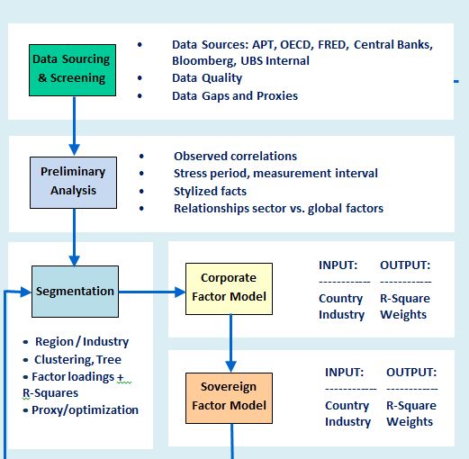
System Dynamics is successfully applied to solve problems in multiple areas. Typically multiple sources of information are used, including numerical data and interviews, to elicit the core information required for modelling a complex system. The advantages of using System Dynamics in Project Management are demonstrated below, but the same benefical features apply to uses in other areas as well.


Project Management in product development, defense, energy and multiple other areas often has to deal with delays and project overruns. As a result problems in schedule and projected costs occur and original planning requires revision. System Dynamics is widely used in Project Management to help assess the source of cost increase and project overruns and to manage projects more effectively.

Large scale projects display a complex dynamics due to many independent components, multiple feedback processes, and non-linear relationships. System Dynamics models are capable to expose such characteristics. 

    • Multiple dependencies among system components are well captured by System Dynamics models and promote transparency about tracing the causal impact of changes throughout the system.
    • Systems exhibit a different behaviour over time. Perturbations to systems for instance cause short-run responses that converge to long-run response after any impact of delays. 
    • Large numbers of feedback relationships for balancing or re-inforcing are a common characterics shown. Tools such as GANTT charts will not solve or even exhibit the impact caused by multiple feedback processes. The System Dynamics approach by comparison is conceptually capbable to incorporate feedback loops and to forecast any impact.
    • Nonlinearity observed in large systems leads to non-proportinal relationships between causes and effects.System Dynamics model incorporate and project non-linear behaviour in the model formulation.


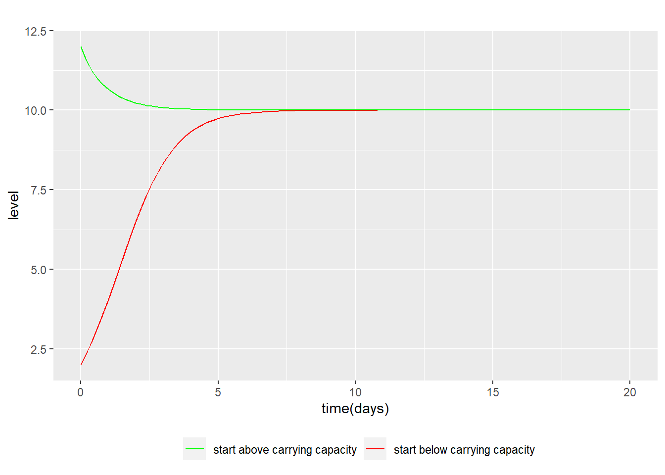
Demonstration of the Logistic Growth Model

Ordinary Differential Equations (ODE) are useful in describing growth phenomena in multiple areas. The logistic equation describes a growth pattern that is commonly observed in a context where competing forces and saturation effects lead to limitations in growth.
To illustrate, consider the growth of company revenues from selling a product until market saturation takes place. For a variable of interest y, its growth is limited by a carrying capacity. Specifically, growth is reduced with higher levels of y due to competing forces that pull the levels towards the carrying capacity. As a result, growth is initially exponential at a growth rate r. However, with increasing levels of y the growth turns negative above a carrying capacity K. The logistic ODE describing this phenomenon is written as. 

\[\normalsize \frac{d\,y}{d\,t} = r \cdot y \cdot (1-\frac{y}{K})\]

Considering two solutions to the logistic equation, each for an initial condition specified by \(y(0)=2\) and \(y=12\). Parameters are specified as \(r=1\) and \(K=10\). Displayed below are two solutions to the logistic equation. For each initial condition the matching solution is shown.


Analytics and Data in Auditing

Details
Insights

Reviewing Analytics and Data - An Outline

Incrasingly more companies and financial institutions base or augment their decision making on data and analytics. For audit to keep pace with expectations, more analytics and advanced technology has to be integrated into the review process. The sampling process traditionally used in reviewing leaves the risk to overlook important review areas such as key transactions, models or business activities. Hence, using advanced analytics for reviewing can have a significant impact on quality and outcome. The review of analytical models renders an area where the use of advanced analytics suggests significant benefits. 

 → READ MORE ...  Guide on Risk-Based approach: Financial Action Task Force (FATF)


Compliance is an area where attempts to prevent money laundering and to establish surveillance over transactions various machine-learning (ML) oriented approaches have become established. Within this context, ML methods are meanwhile commonly used within the context of customer screening. Caveats occur however due large number of false positives as operators have to process all false positives of an outcome run. Clearly, a business objective in this regards is to minimize false positives and thus reduce operational costs involved.  

From the example just sketched it becomes clear that selecting, learning and evaluating ML model is a laborous and complex task with risks of foregone opportunities for performance enhancements due to errors in the model development and validation processes. Auriscon can help in identifying the inconsistencies the development and validaiton approach and point to foregone opportunities to enhance model design and validation.    


Data reviewing has become an ever more important part of technical auditing. As processes, models and transactions become more data intensive the number of variables involved has multiplied. As a result of this trend more data should be analyzed and more trends and patterns are identifiable as part of data auditing. Furthermore, IT tools have emerged to support integration of data managment and machnine learning making thus making it easier for non-IT specialists to analyze and interpret data.


Regulatory expectations on data integrity and governance establish demand for detailed metadata repositories, data lineage and automated data quality checks to be implemented with sufficient granularity and currentness.  Industry standards are set out holistically in the BCBC 239 report with internal reporting, regulatory reporting and management decision systems being in scope.  

Furthermore, institutions are expected to have data quality management and standards in place with data quality indicators and tolerance level attached. 


Consequently, technical leaned audit assignments should incorporate data quality and data governance aspects into the reviewing process.Typical challenges in implementing standars on data quality management are heterogeneous system landscapes where multiple source systems from which data are obtained are used across businesses and functions. Auriscon can help in identifying the inconsistencies and effectivity weaknesses that affecct the data quality measurement and reporting tools.    


 →  READ MORE ...   ECB guide on effective risk data aggregation and risk reporting    


          • Thematic Drivers in Technical Auditing


Model Design

Methodology may have limitations or model design may be incomprehensive leading to bias in model outputs.


Data Quality

Data quality may have weaknesses leading to incomplete, inconsistent or inaccurate data with negative impact on accuracy of model outputs.


Documentation Quality

Poor documentation quality with lack of detail on important model and methodology assumption hinders effective validation and may lead to wrong model use.


Governance Effectiveness

Ineffective governance on thematic aspects such as data, models, IT, risk may lead to breaches with regulatory requirements.


Reviewing Data and Identifying Limitations:

This should include a description of the data used for model build and for model operation. The latter references the data inputs.

Validity of data and quality are key aspects the review should opine on. Aspects of data quality such a missing data or outdated data should receive sufficient attention to summarize data limations under this section. Complications amy arise in the context of feeder models and data filtering and screening processes outside of the actual model development or operation.  

The testing of data quality for model build and life would be suitably expanded on sub topics if data classifications suggest this.  Testing of data quality should also consider the data quality monitoring with respect to relevant data quality dimensions viz. completeness (no missings), accuracy (no outliers), timeliness, controlled data sources, usage monitoring.

The reviewing of suitable and controlled Data Sources links to data integrity requirements. Often, a central data repository is used and checks may cover controls implemented to ensure data consistency across several IT systems. Governance aspects pertaining to definition of Critical Data Elements my have to be considered depending on the scope and the scrutiny of the review.


Reviewing Model Design:

Typically the review part in this section concerns the model assumptions and limitations alongside a description of the model. Theoretical and mathematical exposition should reference literature and classify best practice whenever possible.

In addtion, the calibration process and details should be explained and assessed against potential gaps and weaknesses in relation to model uses.

The audit testing of adequacy of Model Design would be suitably expanded to cover comparisons to industry practice and model benchmarking. 

Robustness of Model Design should stand the test of time and the test of stress. Risk drivers should be captured to the extent to permit model reactivity in times of economic stress.


Reviewing Model Performance:

Reviewing the Performance of the Model is best executed against clear criteria.

Common approach is to set up these criteria before model use and to establish a documented performance monitoring with tresholds on tolerated and alerted breaches of model performance.  

Performance monitoring would capture model use and design issue, as well as issues pertaining to proxy data and model calibration.

The approach to escalation of breaches in model performance should be defined as part of Model Governance. A clear path for escalation reporting should be communicated and documented.


Default Risk in the Trading Book

Details
Insights

The Regulatory Requirements 

The Basel Committee on Banking Supervision (BCBS) replaced the previous Basel 2.5 standards with new standards on Minimum Capital Requirements for Market Risk (FRTB). A revision performed under the Fundamental Review of the Trading Book (FRTB) aims to correct biases in Basel 2.5. As before, a Standardized Approach (SA) and an Internal Model Approach (IMA) apply, Hoqwcwe, this time any regulatory approval for the Internal Model Approach (IMA) is specific and separate for each trading desk. Moreover, Standardized capital has to be calculated on a shadow basis  involving Back-testing and a P&L attribution testing to ensure breaches in the application test criteria are detected. 

Following is an outline of the Default Risk Charge (DRC). Originally imposed by regulatory authorities as the Incremental Risk Charge (IRC) to provision for credit risk losses in the trading book. The DRC metric is defined as a 99.9% VaR over a 1 year horizon, accounting for losses in the trading book due to default and rating migration in credit risky securities. The characterical features of the DRC model have to comply with specific regulatory requirements. 

  • Computed as a 1-year VaR.
  • Only one single jump-to-default risk.
  • Credit risky positions in the trading book covered including listed equities and derivatives.
  • Factor model with two types of systematic factors.
  • Liquidity horizons and constant positions over a 1-year horizon.


The Default Risk Charge Model 

The DRC VaR is calculated from the distribution of simulated portfolio value changes at the 1-year time horizon based on the default / non-default mode. A Factor Model is used to simulate default events. In the Factor Model, an issuer default event at the horizon is detected by comparing the firm’s asset return value r_i at the horizon with a threshold \(c_i=N(p_i)\), using the issuer’s one-year probability of default \(p_i\).

 A firm’s asset return at the 1-year horizon is explained by normal distributed composite factor \(Ψ_i\) and residual \(ϵ_i\). The portion of the total variance of the standardized returns  that is explained by the systematic factors is captured by the R-squared.


\[r_i=√(R_i^2 )⋅Ψ_i+ϵ_i \]

\[with \,\,\, r∼N(μ,Σ)\]

A decomposition of the composite factor in \(j=1,...,M\) systematic factors \(F_j\) is performed in similarity to Moody's GCORR Factor model. Specifically, global factors \(F_(G, j)\) and sectorial factors \(F_(S, j)\) are used to represent systematic factors. Sectorial factors are further partitioned into region, country and industry factors. In addition, company size and credit quality are considered as part of the sectorial dimension. 

Orthogonality of factors ̃\(F_i\) is desirable and obtained from application of principal component analysis (PCA). Specifically, by means of the PCA method the initial correlation matrix \(C\) is decomposed into a diagonal matrix of ordered eigenvalues \(Λ\) and an orthogonal matrix of eigenvectors \(V\). The set of K orthogonal factors is obtained by selecting the eigenvectors associated to the largest K eigenvalues. 


\[C\,=\,V⋅Λ⋅V\]


Capture DRC1


Global factors defined by the set \({F_(G, i) }_((i=1,...,N_G))\) and sectorial factors are defined by the set \({F_(S, i) }_((i=1,...,N_S))\). Furthermore, industry factors \({F_(I, i) }_((i=1,...,N_I))\) , regional factors \({F_(R, i) }_((i=1,...,N_R))\) and the Size factor \(F_Size\) are used, each defined as a sub-set of sectorial factors. Factor weights are obtained from a linear regression of standardized returns on systematic factors.

Measurement of correlations is based on weekly equity returns and weekly sovereign returns with the latter being derived from 5Y CDS spreads. The sample correlation matrix \(C\) is computed from the (N x T) data matrix X of N issuers each with a time series length T at a weekly frequency. The parameters considered are the measurement interval T, the calibration period and the stressed period.


\[C=T^(-1)⋅X⋅X^t\]


Simulation and Valuation

As compared to a single-period model, a multi-period model incorporates the dynamics of default risk over time and addresses the DRC regularity requirement of liquidity horizons. N.B. liquidity horizons for cash equities and derivatives can be shorter than a 1-year capital horizon. Additional consideration is placed on the following:

  • Non-linear impact of derivatives w.r.t. loss from default.
  • Netting long/short to the same obligor has to account for seniority for different instruments.
  • Basis risk between long/short of different obligors must be modelled explicitly.

Simulation method 1: The simulation of correlated default times \(τ_i\) is performed using the distribution of default times \(F_τ (t)\) as determined by the issuer’s PD term-structure \(p_i (t)\) and the returns \(r_i\) as simulated from the factor model.
\[τ_i=F_τ^(-1) (N(r_( i, T)))\]
For each issuer i realizations are drawnb from the composite factor \(Ψ_i\) and the residual \(ϵ_i\) with \(Ψ_i,〖 ϵ〗_i ~ N(0,1)\) and obtain the simulated scenario returns 〖\((r ̂_1,…,r ̂_n)〗_(j=1 ,…,K)\).
A vector of scenario of default times 〖\((τ ̂_1,…,τ ̂_n)〗_(j=1 ,…,K)\) is obtained from applying the standard normal to scenario returns and inverting the default time distribution.

With the assumption of a constant hazard rate \(h ̅_i\) exponential default times with the mean default time \(1/h ̅_i\) are sampled.
\[τ_i=1/(log(1-p_i (T)))∙log(N(r_i))\]
The Gaussian copula representation \(C_(2,Σ)\) of joint default times is
\[P(τ_1≤t_1,〖 τ〗_2≤t_2)=N_2 (N^(-1) [F_(τ_1 ) (t_1 )],〖〖 N〗^(-1) [F〗_(τ_2 ) (t_2 )]))=C_(2,Σ) (F_(τ_1 ) (t_1 ),F_(τ_2 ) (t_2 )])\]

Simulation method 2: Uses the Student -t copula \(C_(k ,Σ,df)\) for k issuers with df degrees of freedom and inputs the same correlation matrix of returns \(Σ\) as used for the Gaussian copula. However, the horizon factor return are modified using a Chi-Square distributed random variable \(X ~ χ^2 (d)\) .
\[r_i=√(df/X)∙[√(R_i^2 )⋅∑_(j=1)^M▒w_(i,j) ⋅F_j+√(1-R_i^2 )⋅ϵ_i ]\]


Capture DRC2

Machine Learning Methods

Details
Insights

bibliothek innovation 2

Advances in Information Technology (IT) based on improvements in hardware and software enabled the success of Machine Learning (ML). Today, the application of robots, automation, and models with capacity to learn from data are commonplace. This makes the tailoring of applications possible to draw insights efficiently from complex and high dimensional data sets.

 The performance of new developed models is evaluated on sample data not used for model training. A reasonable performance of the model on this validation sample would suffice as an indication for acceptable model performance on any new data. The probing of the model on validattion data is a necessary step: high performance on training data may indicate model overfitting leading to a model that is not performing on new data. Overfitting can be traced to noisy data and circumstances where intensive model training leads to an adaption to rare patterns only accommodated in the training data set. 

A consequence of model overfitting is poor performance on new data where the pattern the model has been fitted to is absent. 

Read more: Machine Learning Methods

IFRS 9 and Expected Credit Losses

Details
Insights

JA Edenite

As a result of IFRS9, the IASB demised the Incurred Loss standard and replaced it by the Expected Credit Loss (ECL) standard. IFRS9 accounting require banks to hold provisions for credit losses that are expected to occur, and the amount of provisious is subject to increase for loans whose credit quality has substantially deteriorated. 

The ECL is measued over life of credit risky securities in the banking book. The ECl is a standard that is based on a forward-looking approach with a view on anticipated expected losses. Loss estimation is performed at stages conditional on the loan life cycle.   


Read more: IFRS 9 and Expected Credit Losses

Applications of Scenario Analysis in Finance

Details
Insights

Our company

An important modelling decision faced by risk management is the selection of plausible scenarios to support forward looking risk analysis and stress testing. For example, the computation of Expected Credit Losses (ECL) under IFRS 9 requires an accommodation of suitably devised long-range scenarios.

A common component to applications of Scenario Analysis in Financial Stress Testing is the set-up and use of a framework. The framework provides the linkage between macroeconomic scenarios and risk metrics for the purpose of projecting financial metrics under the mulltiple economic scenarios.  


Vector Autorregression (VAR) is a useful method for analysing macroeconomic and financial data. Specifically, the VAR method permits analysing and accounting for the dependence and dynamics of the macro variables used for scenario building.

 →  READ MORE ...


Scenario Narrative

Stress Testing is well established as a risk management tool across financial institutions. This holds particularly true in in relation to Bank Capital, where regulatory requirements demand that banks adhere to regular internal and external stress testing exercises. A common question of interest to Portfolio and Risk Managers when evaluating the uncertainty of extreme market events is the following:

“How sensitive is my portfolio to losses as a result of macro and financial shocks?”

Macro Stress Testing aids in exploring how hypothetical future shocks deemed to affect the economic and financial environment transmit to the portfolio losses and the income conditions of financial organisations. A major objective of any stress testing exercise is to examine the solvency of and profitability of financial institutions in the advent of crisis. To facilitate this objective the design of the scenarios used in stress testing is therefore required to adapt to the specific risk and portfolio perspective of each organisation. This requirement is facilitated for example by incorporating suitable liquidity and funding shocks into the design of scenarios.

Scenario Design

The scenarios used for macro stress testing should be devised with view on risks that matter. Each financial institutions has a specific risk profile dependent on the prevailing economic and financial conditions over the periods considered. Notheworthy tha stress testinng scenarios are not meant to forecasts of economic conditions in the future!

Starting point for scenario design is the identification of macro and financial risks that could impact negatively on the financial or solvency position of the financial institution. Following the identification of key macro risks and variables with specification of shocks applied to these variables the portfolio impact can be analysed.

Market Risk Stress Testing

Despite the common standards in using Value at Risk (VaR) and Expected Shortfall (ES) metrics, significant residual risks remain due to extreme and random market moves in the risk drivers. Ideally, forward looking scenarios should be evaluated in Market Risk Stress Testing to identify plausible and extreme shocks. However, scenarios based on historical data are often preferred due to the traceability of evidence for identifying shocks.

After the design of suitable scenarios for the core assets a scenario expansion needs to be applied to capture the responses of the non-core assets to the shocks in the drivers. The modelling of the co-dependence between variables under stressed market conditions is essential too. Typically the scenarios provided in regulatory or internal stress tests specify the time path of some key variables only. To exemplify the case for scenario expansion, consider a scenario where GDP growth and inflation change of EU countries is available, but US macro and financial variables are left unspecified.  

Main Menu

  • Home
  • Expertise
    • About Us
    • History
    • Technical Audit
    • Model Development
    • Business Processes
  • Insight Contents
    • IFRS 9 and Expected Credit Losses
    • Applications of Scenario Analysis in Finance
    • Analytics and Data in Auditing
    • Default Risk in the Trading Book
    • Methods of Machine Learning
    • System Dynamics Insights
  • Explore
  • Contact

Consulting Service

  • Business Processes
  • Model Development
  • Technical Audit
  1. You are here:  
  2. Home
  3. Insight Contents
  4. System Dynamics Insights

Contact

AURISCON Ltd
167-169 Great Portland Street
5th Floor
London W1W 5PF
United Kingdom
 
  • +44 (0)7506 456742
  • This email address is being protected from spambots. You need JavaScript enabled to view it.

Company Details

Company No: 11889090

VAT Reg No: 322451830

Copyright © 2023 - 2025 Auriscon Limited.
All rights reserved