The System Dynamics approach was developed as a method for examining systems. A particular aim was to better understand how and when systems fail. The Simulation approach used for System Dynamics has proven to be suitable to obtain valuable insights about the behavioural dynamics of systems and processes. We support in evaluating performance and efficiency of owned systems and processes in:
|
|
|||
|
|
Disclaimer: Data, charts and commentary displayed herein are for information purposes only and do not provide any consulting advice. No information provided in this documentation shall give rise to any liability of Auriscon HK Ltd.
|
|
| System Dynamics: |
|
|
|
|
|
|

|
Auriscon supports: |
|
|
|
|
|
The Applications
System Dynamics provide valuable insights when evaluating long-term behaviour of systems and processes. Applications of System Dynamics span multiple areas, inlcuding Process Change Management, Product Development Planning, and Project Management.
Supply Chain Management enablescompanies to react to a changing business environment by provisioning for having in stock the right products at the right quantities to satisfy customer demand. Among other factors, effectiveness of supply chains is dependent on demand uncertainty, often amplifed by short product life cycles. Reducing instability in the supply chain is therefore important for profitability, Simulation guides in anticipating inventory gaps by testing different scenarios, and by providing input to evaluating and improving inventory processes.
Supply Chains are everywhere!

Inventory Gap and Order Rate
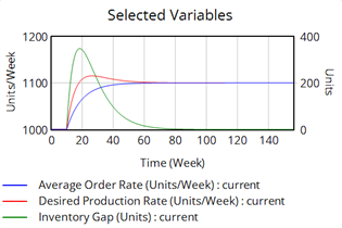
Simulating Inventory Variations
- Anticipating inventory problems.
- Attaining the target inventory performance.
- Responding timely to change in orders and dampening inventory gap oscillations.
- Testing scenarios to support policy updates in Inventory and Supply-Chain management.
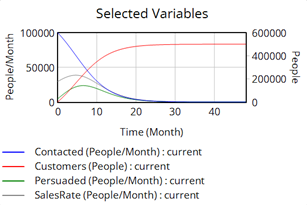
Strategic Planning is a process applied in companies to adapt their decision making to future uncertainties. Effective strategic management therefore helps companies to form a vision and to select the right strategy. at the right time.Different techniques are at disposal to support managers in their decision making. For example, System Dynamics can be used to simulate behavioural pattern in Sales, with customer.behaviour and effects of Marketing simulated to adjust Sales strategies.
Products sold, Happy Sales Team!

Product Sales Behaviour - Modelling of Cause and Effect Relationships
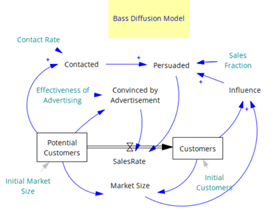
Advertising versus Words-of-Mouth impact on Sales Pattern
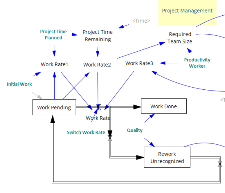
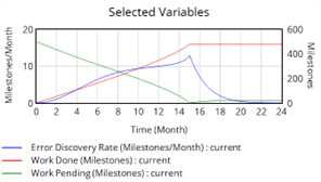
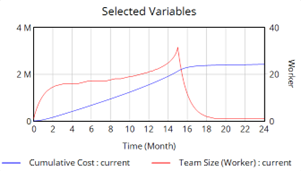
The management of projects with high complexity and uncertainty benefits from the application of System Dynamics. System Dynamics provices a framework for exploring scenarios of dynamic behaviour encountered over the life span of projects. For example, re-work cycles can be integrated into the System Dynamics model to faciliate further insight into delays and project overruns. Root causes in overrun of schedule and projected costs when compared to the original planning can be examined.
Good project planning, Good outcome

Project dynamics - Accounting for re-work cycles and variations in team size
Companies and their Business Processes continously face changes over time. Competitive advantages must be defended against other innovative companies and strategies must be developed to respond to drifts in customer demand. System Dynamics is useful for simulation,of scenarios to test viabiliy of options in Strategy Management. System Dynamics can provide valuable direction for Strategy Management. As a case in point, use of System Dynamics can provide input to assessing a company’s strategic position and evaluating the impact of different strategy options and scenarios. A targeted outcome can be to identify an appropriate business strategy for implementation.
Adjusting business processes to the next business and technology wave

- Used for Change Management simulation.
- Providing insights into feedback processes that determine the behaviour of changed processes.
- Accomplishing the targeted improvement in process performancSupportive of drastic change of the underling process.
lllllllllll