Default Risk in the Trading Book

The Regulatory Requirements 

The Basel Committee on Banking Supervision (BCBS) replaced the previous Basel 2.5 standards with new standards on Minimum Capital Requirements for Market Risk (FRTB). A revision performed under the Fundamental Review of the Trading Book (FRTB) aims to correct biases in Basel 2.5. As before, a Standardized Approach (SA) and an Internal Model Approach (IMA) apply, Hoqwcwe, this time any regulatory approval for the Internal Model Approach (IMA) is specific and separate for each trading desk. Moreover, Standardized capital has to be calculated on a shadow basis  involving Back-testing and a P&L attribution testing to ensure breaches in the application test criteria are detected. 

Following is an outline of the Default Risk Charge (DRC). Originally imposed by regulatory authorities as the Incremental Risk Charge (IRC) to provision for credit risk losses in the trading book. The DRC metric is defined as a 99.9% VaR over a 1 year horizon, accounting for losses in the trading book due to default and rating migration in credit risky securities. The characterical features of the DRC model have to comply with specific regulatory requirements. 

The Default Risk Charge Model 

The DRC VaR is calculated from the distribution of simulated portfolio value changes at the 1-year time horizon based on the default / non-default mode. A Factor Model is used to simulate default events. In the Factor Model, an issuer default event at the horizon is detected by comparing the firm’s asset return value r_i at the horizon with a threshold \(c_i=N(p_i)\), using the issuer’s one-year probability of default \(p_i\).

 A firm’s asset return at the 1-year horizon is explained by normal distributed composite factor \(Ψ_i\) and residual \(ϵ_i\). The portion of the total variance of the standardized returns  that is explained by the systematic factors is captured by the R-squared.

\[r_i=√(R_i^2 )⋅Ψ_i+ϵ_i \]

\[with \,\,\, r∼N(μ,Σ)\]

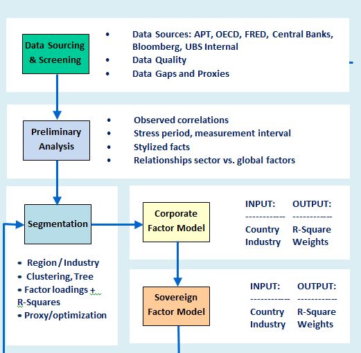
A decomposition of the composite factor in \(j=1,...,M\) systematic factors \(F_j\) is performed in similarity to Moody's GCORR Factor model. Specifically, global factors \(F_(G, j)\) and sectorial factors \(F_(S, j)\) are used to represent systematic factors. Sectorial factors are further partitioned into region, country and industry factors. In addition, company size and credit quality are considered as part of the sectorial dimension. 

Orthogonality of factors ̃\(F_i\) is desirable and obtained from application of principal component analysis (PCA). Specifically, by means of the PCA method the initial correlation matrix \(C\) is decomposed into a diagonal matrix of ordered eigenvalues \(Λ\) and an orthogonal matrix of eigenvectors \(V\). The set of K orthogonal factors is obtained by selecting the eigenvectors associated to the largest K eigenvalues. 

\[C\,=\,V⋅Λ⋅V\]

Global factors defined by the set \({F_(G, i) }_((i=1,...,N_G))\) and sectorial factors are defined by the set \({F_(S, i) }_((i=1,...,N_S))\). Furthermore, industry factors \({F_(I, i) }_((i=1,...,N_I))\) , regional factors \({F_(R, i) }_((i=1,...,N_R))\) and the Size factor \(F_Size\) are used, each defined as a sub-set of sectorial factors. Factor weights are obtained from a linear regression of standardized returns on systematic factors.

Measurement of correlations is based on weekly equity returns and weekly sovereign returns with the latter being derived from 5Y CDS spreads. The sample correlation matrix \(C\) is computed from the (N x T) data matrix X of N issuers each with a time series length T at a weekly frequency. The parameters considered are the measurement interval T, the calibration period and the stressed period.

\[C=T^(-1)⋅X⋅X^t\]

Simulation and Valuation

As compared to a single-period model, a multi-period model incorporates the dynamics of default risk over time and addresses the DRC regularity requirement of liquidity horizons. N.B. liquidity horizons for cash equities and derivatives can be shorter than a 1-year capital horizon. Additional consideration is placed on the following:

• Non-linear impact of derivatives w.r.t. loss from default.
• Netting long/short to the same obligor has to account for seniority for different instruments.
• Basis risk between long/short of different obligors must be modelled explicitly.
  
  

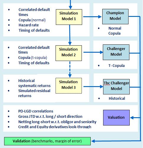
Simulation method 1: The simulation of correlated default times \(τ_i\) is performed using the distribution of default times \(F_τ (t)\) as determined by the issuer’s PD term-structure \(p_i (t)\) and the returns \(r_i\) as simulated from the factor model.
\[τ_i=F_τ^(-1) (N(r_( i, T)))\]
For each issuer i realizations are drawnb from the composite factor \(Ψ_i\) and the residual \(ϵ_i\) with \(Ψ_i,〖 ϵ〗_i ~ N(0,1)\) and obtain the simulated scenario returns 〖\((r ̂_1,…,r ̂_n)〗_(j=1 ,…,K)\).
A vector of scenario of default times 〖\((τ ̂_1,…,τ ̂_n)〗_(j=1 ,…,K)\) is obtained from applying the standard normal to scenario returns and inverting the default time distribution.

With the assumption of a constant hazard rate \(h ̅_i\) exponential default times with the mean default time \(1/h ̅_i\) are sampled.
\[τ_i=1/(log(1-p_i (T)))∙log(N(r_i))\]
The Gaussian copula representation \(C_(2,Σ)\) of joint default times is
\[P(τ_1≤t_1,〖 τ〗_2≤t_2)=N_2 (N^(-1) [F_(τ_1 ) (t_1 )],〖〖 N〗^(-1) [F〗_(τ_2 ) (t_2 )]))=C_(2,Σ) (F_(τ_1 ) (t_1 ),F_(τ_2 ) (t_2 )])\]

Simulation method 2: Uses the Student -t copula \(C_(k ,Σ,df)\) for k issuers with df degrees of freedom and inputs the same correlation matrix of returns \(Σ\) as used for the Gaussian copula. However, the horizon factor return are modified using a Chi-Square distributed random variable \(X ~ χ^2 (d)\) .
\[r_i=√(df/X)∙[√(R_i^2 )⋅∑_(j=1)^M▒w_(i,j) ⋅F_j+√(1-R_i^2 )⋅ϵ_i ]\]