Advances in Information Technology (IT) based on improvements in hardware and software enabled the success of Machine Learning (ML). Today, the application of robots, automation, and models with capacity to learn from data are commonplace. This makes the tailoring of applications possible to draw insights efficiently from complex and high dimensional data sets.
The performance of new developed models is evaluated on sample data not used for model training. A reasonable performance of the model on this validation sample would suffice as an indication for acceptable model performance on any new data. The probing of the model on validattion data is a necessary step: high performance on training data may indicate model overfitting leading to a model that is not performing on new data. Overfitting can be traced to noisy data and circumstances where intensive model training leads to an adaption to rare patterns only accommodated in the training data set.
A consequence of model overfitting is poor performance on new data where the pattern the model has been fitted to is absent.
Techniques used in Machine Learning
The FinTech industry is an illustrative example for a successful business model that has been built on utilizing the advantages of machine learning. Various specialized services are provided by the FinTech industry including robot financial advisors that provide automated advice and assistance in portfolio management, peer to peer lending, crowd funding, fraud detection, mobile payment and access to trading systems for a large retail clientele. In doing so, large number of model configurations are commonly evaluated, leading to robust models that are well adapted to the most recent information in financial data.
Below outlined are some key techniques and illustrations in Machine Learning. Unsurprisingly this outline is not indending to provide a complete picture. The intention is to outline from methodological and informational perspective.
Density Estimation
Representing a large data set compactly is facilitated by Density Estmation. This way, the data set is represented by a density from a parametric family via the density parameter, e.g. mean and variance for Gaussian family. Mixture distributions are more suitable when data are multimodal and not easyliy represented by common base distributions. T
To exemplify, consider a Gaussian Mixture that combines three multivariate Gaussian distributions.
\(p(\textbf{x}, \theta) = \displaystyle\sum_{i=1}^{3} p_i \cdot N(\textbf{x}, \mu_i, \Sigma_i) \)
\( \sum_{i=1}^{3} p_i = 1 \)
Principal Component Analysis
Principal Component Analysis (PCA) belongs to the category of Unsupervised Learning techniques. Unlike Supverised Learning where features and responses are observed, Unsupervised Learning techniques concern situations where only the features are observed. Hence, response prediction is not the objective in Unsupervised Learning, rather it is the classification ob features that renders the objective.
Reducing high dimensional data with many features is useful preliminary stage in data analysis. Analyzing high dimensional data without prior dimensionality reduction can be challenging, if not impossible. For instance, certain features in high dimensional data may be of lesser importance or features may be correlated with each other. Principal Component Analysis (PCA) is a common technique used for dimensionality reduction, permitting to identify latent factors and to analyse data with respect to a few important dimensions.
Clustering
Clustering belongs to the category of Unsupervised Learning techniques and is useful for identifying groups of data that belong together. Precisely, clusteirng classifies data into groups such that the observations falling into one particular cluster have similar features, whereas observations falling in different clusters have different features.
A common approach to clustering is to apply the K-means method. This way data sets are partitioned into K different clusters
Trees
Trees for Regression and Classification problems provide a high visibility for interpretation of results. Moreover, combining a large number of simple Trees for enhancing stability and accuracy of predicted outcomes is possible by means of boosting, bagging and Random Forest methods.
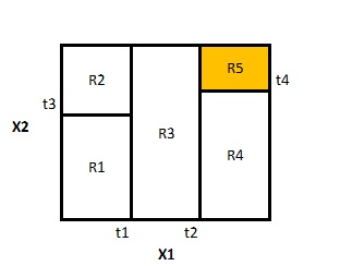
In the application of RegressionTrees one seeks to predict a numerical outcome variable by splitting the space of predictor variables (feature space) into non-overlapping regions. To exemplify, consider a region spanned by two features:
\( Region_5 = \{X_1 \geq threshold_2 \, ,\, X_2 \geq threshold_4\}\)
Such a region represents a terminal leaf in theTree. Each observation with features falling into this region is associated with the same outcome. The outcome variable is calculated as the average outcome for the region.
By comparison, applications of Classification Trees find application in the context of predicting qualitative variables. Another difference to Regression Trees is that the prediction of an observation falling into a certain region (terminal leaf) is calculated as the most commonly occuring categorical value of the predicted variable.
Deep Learning
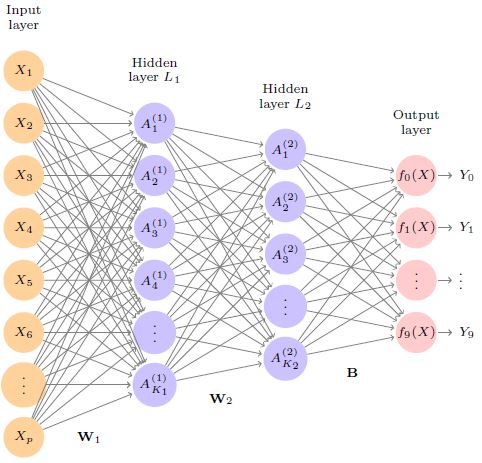
The keywords Deep Learning and Neural Networks are often used interchangeably. Deep Learning has successful applications in Image classification and the areas of speech and text analysis. Based on the Artifical Neural Network (ANN) core methodology, specialisations via Convolutional Neural Networks (CNN) and Recurrent Neural Networks (RNN) have emerged.
In its basic representation, an Artifical Neural Network takes some multi-dimensional input \( X = (X_1,...,X_k) \) to predict a non-linear response \( Y = f(X) \). The input layer of the network is compounded of the predictor variables, aka features. These inputs feed into the hidden layers compounded of activation nodes, whereat activation is modelled by specification of non-lnear functions of the input features \( h_1(X),...,h_m(X) \). The functional form \(g()\) is the same for all activation nodes, only the weight parameters differ for each activation node and are learned as part of the training of the network.
Activation Layer Number of Nodes: 2
Activation Nodes: \(h_j(\textbf{X}) = g(w_{j,0} + \displaystyle\sum_{i=1}^{k} w_{j,i} \cdot X_i) \)
Prediction Node: \(Y = f(\textbf{X}) = \beta_0 + \displaystyle\sum_{i=1}^{m} \beta_i \cdot h_k(\textbf{X}) \)
Sigmoid, Softmax and Heavyside functions are commonly used for specifying the functional form of activation functions. The non-linearity introduced by these functions ensures that interaction effects bewtween features are captured. Fitting a neural network requires estimation of the unknown parameters. As an outcome of fitting, aka training, the parameters are chosen suitably to minimize a loss function. A suitable loss function is the squared error loss computed as the error between the observables \(Y_1,...,Y_n\) and model predicions \(f(X_1),...,f(X_n)\)
Applications of neural networks consists of several hidden layers, each with a modest number of activation nodes. The predicted output can comprise mulitple output variables. Arrangement with multiple outputs are suitable in the context of classification tasks. The method of choice to solve these tasks is the Convolutional Neural Networks (CNN) method. Applications in areas such as image recognition therefore use CNN networks.
The use of .Recurrent Neural Networks (RNN) specialize by design on sequential inputs and time series data. To exemplify, language translation is a case in point whereat both inputs and outputs are sequential. Another example is weather prediction where a time series of observables, e.g. wind speed, rainfall, air pressure, is recorded and fed to the network to predict the weather several days ahead. Financial applications based on using RNNs are plenty and accurate stock price forecasting is a desirable one, albeit accuracy being difficult to achieve. By comparison, forecasting the volume of trading is known to be successfully dealt with by means of RNNs.
Regularization
Linear Regression performs well in situations where the relationship between linear predictor and response is linear, and where the number of observations \(n\) is greater than the number of predictor variables \(p\) . Linear Regression is less suitable however when the number of features exceed the number of observations \(p \gt n \). in which case the Least Square estimates are affected by high variance and hence coefficients become unreliable. Regularization, aka shrinking of estimated coefficients, provides a viable solution to reduce the variance of estimated coefficients. This is achieved by shrinking the estimates towards zero.
In the Ridge Regression method a penalty term is added to the regression sum of squares terms. The penalty term adds the regularization constraint to the least-square estimation. The regularization parameter \(\lambda\) needs to be determined separately. Larger values for \(\lambda\) lead to an increase in regularization. Noteworthy that Ridge includes all predicor variables in the estimated model.
Least-Square-Estimation: \(Y = f(\textbf{X}) = \beta_0 + \displaystyle\sum_{i=1}^{m} \beta_i \cdot h_k(\textbf{X}) \)
Ridge-Estimation: \(Y = f(\textbf{X}) = \beta_0 + \displaystyle\sum_{i=1}^{m} \beta_i \cdot h_k(\textbf{X}) \)
Bayesian Networks
Probabilistic Graphical Models such as Bayesian Networks (BN) provide a suitable framework for complex decision making under uncertainty. Probabilistic Networks have a wide range of applications in areas such as Robot applications, Medical diagnosis and Reliability analysis.
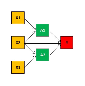
The network structure is represented by a Directed Acyclic Graph (DAG) consisting of nodes and directed arcs. In the DAG, each node`represents a random variable. The directed arcs in the DAG represent dependencies between the variables. Furthermore, each node has a local probability distribution (pdf) associated to it, thereby specifying the dependency between the node and its Parent nodes \(P(node | PAR(node))\) .
Shown below is a DAG representing the Number of Customers a Restaurant can have given the determining factors like Cost of Food, Location and Quality of Food.
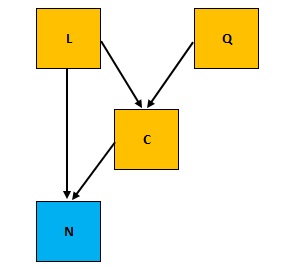
Cost of Food depends on Quality of Food : \(Q \rightarrow C\)
Cost of Food depends on Location of Restaurant: \(L \rightarrow C\)
Number of Customers depends on Cost and Quality: \(C, Q \rightarrow N\)
Reinforcement Learning
Reinforcement Learning (RL) is a technique deemed fundamentally different from Supervised and Unsupervised Learning. The RL model, aka agent, learns through a sequency of interactions with an environment. This permits agents to learn how to act optimally whilst they interact with an environment and collect rewards. Precisly, agents collect positive rewards for benefical actions and negative rewards for adversal actions. The final goal for the agent is to maximize the cumulative reward over time.
At the core of the Reinforcement Learning is the Markov Decision Process (MDP) methodology, by which the agents dynamically interact with an environment through sequences of states, actions and rewards are mathematically described. Another methodology used in the context of Reinforcement Learning is Deep Learning, which has proven to be useful to learn policies from complex representations of data. In Deep Learning mode, the state variables input the network and the output of the network provides the solution for the policy.
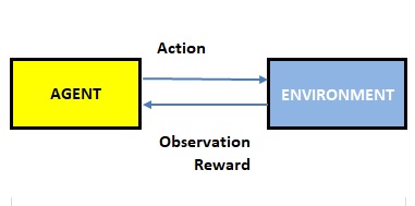
Rewards can be disclosed after each action, or alternatively, after completion of an episode. The latter approach is exemplified by a chess game, where the reward is acknowledged after the game. To win the game, the agent has to learn from the result of the actions via the feedback obtained from the environment.
Current State : \(S_t\)
Action: \( A_t\)
Observation, Next State: \(S_{t+1}\)
Reward: \(R_{t+1}\)
Sequence of Interactions: \((S_1, A_1, R_2) \, \rightarrow \, (S_2, A_2, R_3) \, \rightarrow \, \cdot \cdot \cdot\)