Bayesian Networks Primer
A primer on model building and use of Bayesian Networks
![]() Disclaimer: Data, charts and commentary displayed herein are for information purposes only and do not provide any consulting advice. No information provided in this documentation shall give rise to any liability of Auriscon Ltd.
Disclaimer: Data, charts and commentary displayed herein are for information purposes only and do not provide any consulting advice. No information provided in this documentation shall give rise to any liability of Auriscon Ltd.
Overview
Introducing Bayesian Networks
Bayesian Networks have proven usefulness for machine learning and expert systems in various areas such as speech recognition, signal processing, bioinformatics, and medical diagnosis. Decision making under uncertainty often has to consider a large number of factors which are specified as part of the network structure (graph topology) and the parameters in the Bayesian Network. In many practical settings the parameters of the local probability distributions are unknown and one needs to estimate these from data. Learning the network structure is considered more difficult than learning the parameters even though the graph structure can be elicited based on expert guidance.
Bayesian Networks (BN) belong to the type of Probabilistic Graphical Models and provide a suitable framework to aid complex decision making with a wide range of applications. The structure of a Bayesian Network is represented by a Directed Acyclic Graph (DAG) consisting of nodes and directed edges Precisely, each node`in the network represents a random variable and edges between nodes represent dependencies. Furthermore, each node has a local probability distribution (pdf) associated to it whereby dependencies are modeled.The local probability distributions associated to each node have incorporated the information of parent nodes and expressed in the functional form \(\small P(node \, | \, Par(node))\). With the following blog a brief primer on Bayesian Networks is presented to interested parties.
- Dependencies between variables
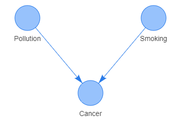
Dependencies between nodes (random variables) in Bayesian Networks are indicated by directed edges. A directed edge between two nodes \(A\rightarrow B\) displays the direction from the cause to effect (symptom). Shown in the graph below is the dependency between the symptom of having cancer and a possible causes of high pollution and smoking habit. Noteworthy that all direct dependencies are represented by arcs.
- Indirect dependencies
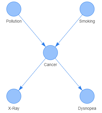
An indirect dependency is a path between two nodes that is blocked by another node. To exemplify, consider the previous example of having cancer which may be indicated by having a positive X-ray result or which may lead to having Dysnopea diagnosed. In this example smoking can’t effect Dysnopea directly without having caused cancer in the first place.
- Inferring probabilities for variables
Inference in Bayesian Networks refers to the process of of estimating probabilities, namely the conditional probabilities associated to the nodes (variables). The inference is based on evidence about variables. An example is illustrated below: by updating the node having positive X-Ray (X) with the value True the probability for having Cancer (C) can be inferred. The conditional probabilities of having a a positive X-Ray result, namely \(\small P(X\, |\, C = True)\) and \(\small P(X\, |\, C = False)\), are of interest. Inference in this example is rendered by updating our belief on having Cancer given the outcome of a postive X-Ray result.
\[\small P(C = True \,|\, X = True) = \frac{P(X = True , C = True) \cdot P(C = True)}{P(X = True)}\] \[ \small P(C = False| X = True) = \frac{P(X = True , C = False) \cdot P(C = True)}{P(X = True)}\] \[ \small P(C = True) = \frac{P(X = True)}{P(X = True , C = True) + P(X = True , C = False))}\]
Noteworthy that probabilities can be elicited from either the knowledge of experts or estimated from data. Determining probabilities with the help of subject matter experts can be a time consuming approach however. Therefore, estimating probabilities from data is preferable and helps to avoid bias in estimates. By estimating the local probabilities a conditional probability table P(Y|X) is attached to each node in the network.
- Conditional independence between variables
Nodes that are directly connected via an edge depend directly on each other in terms of probability. By comparison, nodes that are not directly connected via an edge are independent conditional on some other nodes. The Bayesian network structure expresses graphically conditional independence relationships among variables through appearance of certain graphical patterns.
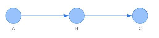
Sequential: a cause-effect path connecting three nodes sequentially \(\small A\rightarrow B\rightarrow C\). This pattern represents a conditional independence relation. Knowing that an event has occurred in the parent node B leads to an effect on the child node C irrespective of whether node A has been affected by an event. The conditional independence relation is written as \(\small C\bot A\,|\,B\), or alternatively written as \(P\small (C\,|\,A,\,B)\,=\,P(C\,|\,B)\).

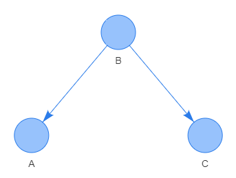
Reversed V-pattern: a common cause path connecting three nodes by a reversed V-pattern \(\small B\leftarrow A\rightarrow C\). An event that has occurred in the parent node A leads to an effect on child nodes B and C. irrespective of whether node A has been affected by an event. This pattern represents a conditional independence since knowing that common cause A has occurred determines the event C irrespective of what event in node B has occurred. The conditional independence relation is written as \(\small B\bot C\,|\,A\), or alternatively written as \(\small P(C\,|\,A,\,B)=P(C\,|\,A)\).
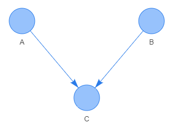
V-pattern: a common effect path connecting three nodes by a V-pattern \(\small A\rightarrow C\leftarrow B\). This pattern represents conditional independence since knowing that common effect C has occurred determines not uniquely the event in node B irrespective of what event has occurred in node A. This conditional independence relation is written as \(\small A\not{\bot} B\,|\,C\), or alternatively written as \(\small P(C\,|\,A,\,B)=P(C\,|\,A)\).
Finally, the notion of conditional independence in Bayesian Networks can be extended to larger sets of nodes. A set of nodes \(\small Z_1, ..., Z_i\) is said to be conditionally independent of another set of nodes \(\small X_1, ..., X_j\) given a set of evidence nodes \(\small Y_1, ..., Y_k\). Precisely, one states that there is d-separation between the set of nodes in X and the set of nodes in Z.
- Factorizing the global probability distribution
Conditional independence relationships in Bayesian Networks are important for reducing the number of parameters required for specification. Since conditional probability distribution (CPD) at each node depend only on its parent nodes, a significant reduction in parameters is achieved for both local and global distributions.
A Bayesian Network that consists of multiple nodes (variables) is characterized by many local probability distributions each attached to one node. For discrete random variables each local probability distribution is represented by a table thereby listing the local conditional probabilities for node value instantiations given the combinations of parent node values.
The global probability distribution, aka joint probability distribution (JPD), is represented by a factorization into local probability distributions. As a result, the high-dimensional global distribution for \(\small X_1,..,X_n\) is expressed through a set of local distributions \(\small P(X_i \, | \, Par X_i)\) for \(\small i=1,..,K\) with \(\small K \le n\).
\[\small P(X_1,...,X_n) = \prod_{i=0}^{K} \, P(X_i \, | \, Par X_i)\]
Demonstrating a Bayesian Network
From the graph displayed below the local distribution functions are set and the global distribution function can be derived suit.
\[\small P(A,B,C,D,E) = P(A) \,\cdot\,P(B) \,\cdot\,P(C \, | \, A, B) \,\cdot\,P(D\, | \,C) \,\cdot\,P(E \, | \, C) \,\cdot\,P(F \, | \, D \,, \, E)\] Given the DAG structure is already specified as shown, what remains in the Learning stage is estimating probabilities. We next assume the Learning stage has been completed already and that the probabilities are determined as follows:
Applications of Bayesian Networks
UNDER CONSTRUCTION
Glossary
-
DAGdenotes a Directed Acyclic Graph, that is a graphs without cycles, i.e. a path starting from one node cannot end at the same node. -
Nodesrepresent the random variables in graphs. -
Ancestorrepresents a parent node to other nodes in a chain of nodes since it comes first. By contrast,descendantrepresents a child node in a chain of nodes since it comes last. In a graph, root nodes with no ancestors represent root causes whereas leaf nodes with not descendants represent final effects. -
Arcs, aka edges, visualize the direction of cause-effect relationships or probabilistic dependencies between pairs of nodes in the graph. If there is no arc between two nodes the corresponding variables are either independent or conditionally independent. -
Conditional probability distributions(CPD) represent the probability of event X1 given that events for X2, X3, etc. have occurred. -
P(node | Par(node)) is the
local distributionattached to a node. The local distribution is given by a conditional distribution, where Par(node) denotes the parent nodes of the node. -
P(A1,A2,A3,,…,An) denotes the
global distributionattached to all variables in the Bayesian network.