Insights

The ongoing trend in using quantitative models for decision making prompted institutions and regulatory authorities to establish stricter rules on model risk management. Examples of this continuing expansion can be found in various model using areas e.g. the use of algorithms for trade execution in Securities Trading, the use of decision models in Credit Risk Analytics. Financial risk areas like Credit, Market or Compliance Risk entail model use cases with exposure to Model Risk. 

To ensure al lnternal Rating Based (IRB) models are adequate and address regulatory requirements, IRB models are subject to a regular validation cycle. With emphasis given to a thorough model backtesting and benchmarking, annual validations are commonly supplemented by the results of model monitoring and the use of external data sources too.

The Regulatory Requirements 

The Basel Committee on Banking Supervision (BCBS) replaced the previous Basel 2.5 standards with new standards on Minimum Capital Requirements for Market Risk (FRTB). A revision performed under the Fundamental Review of the Trading Book (FRTB) aims to correct biases in Basel 2.5. As before, a Standardized Approach (SA) and an Internal Model Approach (IMA) apply, Hoqwcwe, this time any regulatory approval for the Internal Model Approach (IMA) is specific and separate for each trading desk. Moreover, Standardized capital has to be calculated on a shadow basis  involving Back-testing and a P&L attribution testing to ensure breaches in the application test criteria are detected. 

Following is an outline of the Default Risk Charge (DRC). Originally imposed by regulatory authorities as the Incremental Risk Charge (IRC) to provision for credit risk losses in the trading book. The DRC metric is defined as a 99.9% VaR over a 1 year horizon, accounting for losses in the trading book due to default and rating migration in credit risky securities. The characterical features of the DRC model have to comply with specific regulatory requirements. 

The Default Risk Charge Model 

The DRC VaR is calculated from the distribution of simulated portfolio value changes at the 1-year time horizon based on the default / non-default mode. A Factor Model is used to simulate default events. In the Factor Model, an issuer default event at the horizon is detected by comparing the firm’s asset return value r_i at the horizon with a threshold \(c_i=N(p_i)\), using the issuer’s one-year probability of default \(p_i\).

 A firm’s asset return at the 1-year horizon is explained by normal distributed composite factor \(Ψ_i\) and residual \(ϵ_i\). The portion of the total variance of the standardized returns  that is explained by the systematic factors is captured by the R-squared.

\[r_i=√(R_i^2 )⋅Ψ_i+ϵ_i \]

\[with \,\,\, r∼N(μ,Σ)\]

A decomposition of the composite factor in \(j=1,...,M\) systematic factors \(F_j\) is performed in similarity to Moody's GCORR Factor model. Specifically, global factors \(F_(G, j)\) and sectorial factors \(F_(S, j)\) are used to represent systematic factors. Sectorial factors are further partitioned into region, country and industry factors. In addition, company size and credit quality are considered as part of the sectorial dimension. 

Orthogonality of factors ̃\(F_i\) is desirable and obtained from application of principal component analysis (PCA). Specifically, by means of the PCA method the initial correlation matrix \(C\) is decomposed into a diagonal matrix of ordered eigenvalues \(Λ\) and an orthogonal matrix of eigenvectors \(V\). The set of K orthogonal factors is obtained by selecting the eigenvectors associated to the largest K eigenvalues. 

\[C\,=\,V⋅Λ⋅V\]

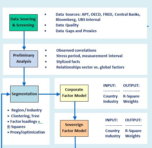
Global factors defined by the set \({F_(G, i) }_((i=1,...,N_G))\) and sectorial factors are defined by the set \({F_(S, i) }_((i=1,...,N_S))\). Furthermore, industry factors \({F_(I, i) }_((i=1,...,N_I))\) , regional factors \({F_(R, i) }_((i=1,...,N_R))\) and the Size factor \(F_Size\) are used, each defined as a sub-set of sectorial factors. Factor weights are obtained from a linear regression of standardized returns on systematic factors.

Measurement of correlations is based on weekly equity returns and weekly sovereign returns with the latter being derived from 5Y CDS spreads. The sample correlation matrix \(C\) is computed from the (N x T) data matrix X of N issuers each with a time series length T at a weekly frequency. The parameters considered are the measurement interval T, the calibration period and the stressed period.

\[C=T^(-1)⋅X⋅X^t\]

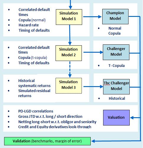
Simulation and Valuation

As compared to a single-period model, a multi-period model incorporates the dynamics of default risk over time and addresses the DRC regularity requirement of liquidity horizons. N.B. liquidity horizons for cash equities and derivatives can be shorter than a 1-year capital horizon. Additional consideration is placed on the following:

• Non-linear impact of derivatives w.r.t. loss from default.
• Netting long/short to the same obligor has to account for seniority for different instruments.
• Basis risk between long/short of different obligors must be modelled explicitly.
  
  

Simulation method 1: The simulation of correlated default times \(τ_i\) is performed using the distribution of default times \(F_τ (t)\) as determined by the issuer’s PD term-structure \(p_i (t)\) and the returns \(r_i\) as simulated from the factor model.
\[τ_i=F_τ^(-1) (N(r_( i, T)))\]
For each issuer i realizations are drawnb from the composite factor \(Ψ_i\) and the residual \(ϵ_i\) with \(Ψ_i,〖 ϵ〗_i ~ N(0,1)\) and obtain the simulated scenario returns 〖\((r ̂_1,…,r ̂_n)〗_(j=1 ,…,K)\).
A vector of scenario of default times 〖\((τ ̂_1,…,τ ̂_n)〗_(j=1 ,…,K)\) is obtained from applying the standard normal to scenario returns and inverting the default time distribution.

With the assumption of a constant hazard rate \(h ̅_i\) exponential default times with the mean default time \(1/h ̅_i\) are sampled.
\[τ_i=1/(log(1-p_i (T)))∙log(N(r_i))\]
The Gaussian copula representation \(C_(2,Σ)\) of joint default times is
\[P(τ_1≤t_1,〖 τ〗_2≤t_2)=N_2 (N^(-1) [F_(τ_1 ) (t_1 )],〖〖 N〗^(-1) [F〗_(τ_2 ) (t_2 )]))=C_(2,Σ) (F_(τ_1 ) (t_1 ),F_(τ_2 ) (t_2 )])\]

Simulation method 2: Uses the Student -t copula \(C_(k ,Σ,df)\) for k issuers with df degrees of freedom and inputs the same correlation matrix of returns \(Σ\) as used for the Gaussian copula. However, the horizon factor return are modified using a Chi-Square distributed random variable \(X ~ χ^2 (d)\) .
\[r_i=√(df/X)∙[√(R_i^2 )⋅∑_(j=1)^M▒w_(i,j) ⋅F_j+√(1-R_i^2 )⋅ϵ_i ]\]

Advances in Information Technology (IT) based on improvements in hardware and software enabled the success of Machine Learning (ML). Today, the application of robots, automation, and models with capacity to learn from data are commonplace. This makes a tailoring of applications possible for inferring insights and for analyzing complex and high dimensional data sets. The FinTech industry is an illustrative example of a successful business model that has been built on utilizing the advantages of machine learning. 

The Despite advantages gained through application of Machine Learning, one has to be cautious of the consequences of model overvitting thouugh. Overfiiting occurs where the performed of the model is excellent of the training data, but fails on real-world data not used for model calibration. 

A subjective list of Machine Learning methods selected for use in Credit Analytics is outlined next.

The International Accounting Standards Board IASB demised the IAS39 Incurred Loss standard and replaced it by the IFRS9 Expected Credit Loss (ECL) standard put in force in 2018. IFRS9 accounting requires banks to hold provisions for credit losses that are expected to occur. The amount of proviisions is dependent on a staged methodology, which includes increasing provisions for loans whose credit quality has substantially deteriorated. 

The ECL is calculated for securities in the banking book based on a forward-looking approach with a view on expected losses. Loss estimation is performed at stages recognizing any decreased credit quality and impairment for stages 2 and 3.   

An important modelling decision faced by risk management is the selection of plausible scenarios to support forward looking risk analysis and stress testing. For example, the computation of Expected Credit Losses (ECL) under IFRS 9 requires an accommodation of suitably devised long-range scenarios.

A common component to applications of Scenario Analysis in Financial Stress Testing is the set-up and use of a framework. The framework provides the linkage between macroeconomic scenarios and risk metrics for the purpose of projecting financial metrics under the mulltiple economic scenarios.  

Scenario Narrative

Stress Testing is well established as a risk management tool across financial institutions. This holds particularly true in in relation to Bank Capital, where regulatory requirements demand that banks adhere to regular internal and external stress testing exercises. A common question of interest to Portfolio and Risk Managers when evaluating the uncertainty of extreme market events is the following:

“How sensitive is my portfolio to losses as a result of macro and financial shocks?”

Macro Stress Testing aids in exploring how hypothetical future shocks deemed to affect the economic and financial environment transmit to the portfolio losses and the income conditions of financial organisations. A major objective of any stress testing exercise is to examine the solvency of and profitability of financial institutions in the advent of crisis. To facilitate this objective the design of the scenarios used in stress testing is therefore required to adapt to the specific risk and portfolio perspective of each organisation. This requirement is facilitated for example by incorporating suitable liquidity and funding shocks into the design of scenarios.

Scenario Design

The scenarios used for macro stress testing should be devised with view on risks that matter. Each financial institutions has a specific risk profile dependent on the prevailing economic and financial conditions over the periods considered. Notheworthy tha stress testinng scenarios are not meant to forecasts of economic conditions in the future!

Starting point for scenario design is the identification of macro and financial risks that could impact negatively on the financial or solvency position of the financial institution. Following the identification of key macro risks and variables with specification of shocks applied to these variables the portfolio impact can be analysed.

Market Risk Stress Testing

Despite the common standards in using Value at Risk (VaR) and Expected Shortfall (ES) metrics, significant residual risks remain due to extreme and random market moves in the risk drivers. Ideally, forward looking scenarios should be evaluated in Market Risk Stress Testing to identify plausible and extreme shocks. However, scenarios based on historical data are often preferred due to the traceability of evidence for identifying shocks.

After the design of suitable scenarios for the core assets a scenario expansion needs to be applied to capture the responses of the non-core assets to the shocks in the drivers. The modelling of the co-dependence between variables under stressed market conditions is essential too. Typically the scenarios provided in regulatory or internal stress tests specify the time path of some key variables only. To exemplify the case for scenario expansion, consider a scenario where GDP growth and inflation change of EU countries is available, but US macro and financial variables are left unspecified.